Principal Component Analysis on implied volatility surfaces

Introduction

In this post, I provide a summary of a project I completed during my undergraduate degree at McGill University. The full report is available on my GitHub here, but this post aims to distill the key points for quick understanding.

The project focuses on applying Principal Component Analysis (PCA) to the implied volatility surface of US Equity Options, inspired by Doris Dobi’s thesis, “Modelling Systematic Risk in the Options Market”. While the original paper emphasizes re-interpolation, my project explores the implications for portfolio construction and extends the research by evaluating various principal component selection methodologies through a simulation study. Key references include:

1. Doris Dobi. Modeling Systemic Risk in The Options Market. PhD thesis, New York University, May 2014.
2. Pedro R. Peres-Neto, Donald A. Jackson, and Keith M. Somers. How many principal components? stopping rules for determining the number of non-trivial axes revisited. Computational Statistics Data Analysis, 49(4):974–997, 2005.
3. Irene Aldridge and Marco Avellaneda. Big Data Science in Finance. John Wiley & Sons, Inc., 2021.

Options and Implied Volatility Surfaces

The dataset focuses on U.S. equity options, specifically those on equities listed in the S&P 500. The key metric analyzed is implied volatility, which reflects the market’s expectation of future realized volatility of the underlying security. Implied volatility is derived by solving for the volatility parameter in the Black-Scholes model, given observed market prices.

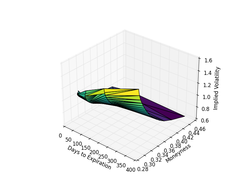
The implied volatility surface is parameterized by time to expiration and delta (a measure of the option’s sensitivity to the underlying asset’s price). Below is an example of an implied volatility surface for AAPL options.

Data Acquisition

Daily equity call options data from August 31, 2004, to August 31, 2013, was obtained from OptionsMetrics, with time to expirations of 30, 91, 182, and 365 days, and delta ranging from 20 to 85. Daily prices for the underlying securities were sourced from CRSP.

Applying Principal Component Analysis

A Review of the Mathematics

Principal Component Analysis (PCA) is a dimensionality reduction technique that constructs new variables (principal components) as linear combinations of the original variables. The goal is to retain as much variance as possible while reducing the number of dimensions. The principal components are orthogonal and ordered such that the first component explains the maximum variance.

Given a dataset \(X\) with \(n\) observations and \(p\) variables, PCA seeks to find a set of orthogonal vectors \(w_i\) such that the linear combinations \(Y_i = w_i^T X\) maximize the variance of the projected data. This is equivalent to solving the following optimization problem:

\[\text{Maximize } \text{Var}(Y_i) = w_i^T \Sigma w_i\]

subject to the constraint \(w_i^T w_i = 1\), where \(\Sigma\) is the covariance matrix of \(X\).

The solution to this problem is obtained by solving the eigenvalue problem:

\[\Sigma w_i = \lambda_i w_i\]

where \(\lambda_i\) is the eigenvalue corresponding to the \(i\)-th principal component, and \(w_i\) is the corresponding eigenvector. The eigenvalues \(\lambda_i\) represent the amount of variance explained by each principal component, and the eigenvectors \(w_i\) represent the weights of the original variables in the principal components.

The proportion of variance explained by the \(k\)-th principal component is given by:

\[\text{Proportion of Variance Explained} = \frac{\lambda_k}{\sum_{i=1}^p \lambda_i}\]

Key assumptions/properties of PCA include:

1. Linearity: Relationships between variables are linear.
2. Orthogonality: Principal components are orthogonal.
3. Scale Variance: PCA is sensitive to the scale of the data.

Two Methods for Applying PCA

In this project, PCA was applied to the implied volatility surface using two different methods: non-coupled and coupled. The key difference between these methods lies in whether the returns of the underlying asset are included in the analysis.

Method 1: Non-Coupled

In the non-coupled method, PCA is applied solely to the implied volatility surface without incorporating the returns of the underlying asset. The implied volatility surface is constructed using options data with different maturities (30, 91, 182, and 365 days) and deltas (ranging from 20 to 85). The data is organized into a matrix where each row represents a date, and each column represents a combination of delta and maturity. The matrix is then transposed, and row-wise log returns are calculated before applying PCA.

Key Results for Non-Coupled Method:

• The first principal component dominates, explaining 84% of the variance for Apple (AAPL).
• The first eigenvalue is significantly larger than the others, with an average of 36.5 across all S&P 500 constituents.
• The first principal component weights positively and nearly equally across all factors, with the highest weights at 45, 50, 55, and 60 delta for 91 and 182 days.
• The second principal component contrasts shorter-term (30 days) and longer-term (365 days) options.

Method 2: Coupled

In the coupled method, PCA is applied to both the implied volatility surface and the returns of the underlying asset. This method includes an additional column in the data matrix representing the price of the underlying asset. The same preprocessing steps (transposing and calculating log returns) are applied before performing PCA.

Key Results for Coupled Method:

• The first principal component still dominates, but it now contrasts the implied volatility surface with the price of the underlying asset.
• The first eigenvalue explains slightly less variance compared to the non-coupled method, with an average of 33.
• The second principal component continues to contrast shorter-term (30 days) and longer-term (365 days) options.
• The inclusion of the underlying asset’s returns provides little additional explanatory power, as the implied volatility surface already accounts for changes in the asset’s price.

Selecting Principal Components

The project explores two main methods for selecting the number of principal components to retain: Marchenko-Pastur and Tracy-Widom.

Marchenko-Pastur Law

The Marchenko-Pastur Law describes the asymptotic behavior of the eigenvalues of large random matrices. It is used to distinguish between significant eigenvalues and those that can be attributed to noise.

Statement: Consider an \(M \times N\) random matrix \(X\) with i.i.d. entries having mean 0 and finite variance. The eigenvalues of the sample covariance matrix \(Y_N = \frac{1}{N} XX^T\) follow a limiting distribution as $$M, N \to \infty \text{ with } \frac{M}{N} \to \Lambda \in (0, \infty)$$

The density of the eigenvalues is given by:

\(\mu(A) = \begin{cases} (1 - \frac{1}{\Lambda})1_{0 \in A} + v(A) & \text{if } \Lambda > 1 \\ v(A) & \text{if } 0 \leq \Lambda \leq 1 \end{cases}\) where \(v(A)\) is the Marchenko-Pastur density:

\[dv(x) = \frac{1}{2\pi\sigma^2} \frac{\sqrt{(\lambda_+ - x)(x - \lambda_-)}}{x\Lambda} 1_{[\lambda_-, \lambda_+]} dx\]

with \(\lambda_{\pm} = \sigma^2 (1 \pm \sqrt{\Lambda})^2\)

Application:

Eigenvalues below \(\lambda_+\) are considered noise and are discarded. For example, in the non-coupled method, the threshold \(\lambda_+\) for Apple was calculated as:

\[\lambda_+ = \left(1 + \sqrt{\frac{52}{2266}}\right)^2 = 1.326\]

Tracy-Widom Distribution

The Tracy-Widom Distribution describes the distribution of the largest eigenvalue of a random correlation matrix. It is used to determine whether the largest eigenvalue is statistically significant.

Statement: The Tracy-Widom distribution applies to Gaussian ensembles (GOE, GUE, GSE) and is defined in terms of the Painlevé II differential equation:

\[q''(s) = sq(s) + 2q(s)^3\]

with boundary condition \(q(s) \sim \text{Ai}(s)\) as \(s \to \infty\), where \(\text{Ai}(s)\) is the Airy function. The distribution for the Gaussian Orthogonal Ensemble (GOE, \(\beta = 1\)) is given by:

\[F_1(s) = \exp\left(-\frac{1}{2} \int_s^\infty q(x) dx\right) \left(F_2(s)\right)^{\frac{1}{2}}\]

where \(F_2(s) = \exp\left(-\int_s^\infty (x - s)^2 q(x)^2 dx\right)\).

Application:

Eigenvalues exceeding the simulated Tracy-Widom threshold are retained as significant. For example, in the coupled method, the Tracy-Widom distribution was used to retain 11 components for the non-coupled method and 77 components for the coupled method.

Tables from the Original Report

Below are some key tables from the original report that summarize the results of the PCA decomposition and the selection of principal components:

Table 1: Highest and Lowest Leading Eigenvalues (Non-Coupled Method)

Ticker	Highest EV1	Ticker	Lowest EV1
JPM	0.888	WEC	0.395
GS	0.881	PNW	0.405
BAC	0.879	NLSN	0.409
MS	0.864	ES	0.417
ICE	0.859	KMI	0.445

Table 2: Number of Components Retained by Method and Rule

Method	Non-Coupled	Coupled
Parallel Analysis	415	2265
Permutation Eigenvalues	11	110
Permutation Eigenvalues % Var.	11	110
Permutation Eigenvalues Ratio	155	807
Permutation Eigenvalues Diff	34	222
Kaiser Guttman	51	465
Random Avg Parallel Analysis	11	110
Random Avg Perm.	11	110
Permutation Eigenvectors	415	2266
Marchenko-Pastur	11	68
Tracy-Widom	11	77

Evaluating Selection Methods

A simulation study was conducted to evaluate various principal component selection methods, including:

• Parallel Analysis: A Monte Carlo approach comparing observed eigenvalues to those from simulated data.
• Randomization Based on Eigenvalues: Permutation tests to determine significant eigenvalues.
• Kaiser-Guttman Rule: Retains components with eigenvalues greater than 1.
• Average under Parallel Analysis: Retains components with eigenvalues greater than the average from parallel analysis.

Results showed that methods like Marchenko-Pastur and Tracy-Widom performed well, particularly for larger datasets, while simpler methods like Kaiser-Guttman struggled with larger dimensions. This highlights the importance of selecting appropriate methods based on the dataset’s size and structure.

Conclusion and Extensions

The project demonstrated the effectiveness of PCA in reducing the dimensionality of implied volatility surfaces and provided insights into portfolio construction by identifying systematic risk factors. Future extensions could include:

• Further exploration of classification methods for systematic risk.
• Expanding the analysis to a larger dataset, including more equities.
• Incorporating additional firm-specific variables, such as trading volume, into the PCA.

All code used in this project is available upon request.