Eigenportfolios: Can We Find the Market from the Data Itself?

If you ask someone what “the market” is they’ll usually point to an index such as the S&P 500. But this choice of “the market” is inherently human - someone, S&P in our example, decided which companies belong, and as a result which don’t belong in the index, how they should be weighted, how they should be rebalanced and much more. In 2026, this seemingly well defined task has gotten even more attention with the debate around the inclusion of large IPOs such as $SPCX proving to not be agreeable across index providers.

These are hard decisions, and I’m certainly not qualified enough to have any input on what their methodologies should or shouldn’t be; so I’ll stick to what I do know, math

The central question of the topic of this post is: What if instead we let the data tell us what the dominant common factor in a set of asset returns actually is, with no index, no benchmark, and no prior assumptions about what “the market” should look like? To do this, we’ll build a purely statistical object — an eigenportfolio — out of nothing but the covariance structure of a handful of ETF returns, and see whether it rediscovers something we already recognize.

Why the Covariance Matrix Is the Right Starting Point

If we want to find co-movement in returns without imposing a structure ourselves, the natural object to study is the covariance matrix \(\Sigma\) of asset returns. The covariance matrix captures, pairwise, how every asset moves relative to every other, and critically, it has a mathematical property that makes it decomposable in a very clean way: it’s positive semi-definite (PSD).

Concretely, a matrix, call it \(\Sigma\) is PSD if

\[x^{T}\Sigma x \ge 0 \quad \forall x \in \mathbb{R}^{n}\]

which is easy to show directly from the definition of covariance. Let \(X\) be our vector of asset returns. Then:

\[\begin{align} x^{T}\Sigma x & = x^{T}E[(X-E[X])(X-E[X])^{T}]x \\ & = E[x^{T}(X-E[X])(X-E[X])^{T}x] \\ & = E[(x^{T}(X-E[X]))^2] \ge 0 \end{align}\]

since the expectation of a squared quantity can never be negative.

Why does this matter for us? A symmetric PSD matrix like \(\Sigma\) can always be written as

\[\Sigma = U\Lambda U^{T}\]

where \(U\) is orthogonal (its columns are orthonormal eigenvectors) and \(\Lambda\) is diagonal with non-negative eigenvalues. This is the spectral decomposition of \(\Sigma\), and it’s the machinery underneath everything that follows: it guarantees we can split the variance in our returns into a set of orthogonal (uncorrelated) directions, each with a well-defined, non-negative amount of variance attached to it. That guarantee is what makes the next step PCA mathematically sound.

What PCA Actually Gives Us

Principal Component Analysis (PCA) takes that spectral decomposition and gives it a statistical interpretation:

• Each eigenvector of \(\Sigma\) defines a direction in “asset-return space”, that is, a specific linear combination of assets.
• The corresponding eigenvalue tells us how much of the total variance in the data is explained by moving along that direction.
• Because the eigenvectors are orthogonal, these directions are uncorrelated with each other and each one captures a distinct, non-overlapping slice of the market’s variance.

Sorting components by eigenvalue size gives us a ranked list of “what’s driving co-movement,” from most important to least. If there’s a single dominant factor behind a group of asset returns, we’d expect to see it show up as an outsized first eigenvalue, and a first eigenvector whose weights look, in some sense, like “the market.”

To test this, we ran PCA on daily returns for a set of industry ETFs, 2024-01-01 to 2026-01-01. The loadings of the first 2, principal components are shown below:

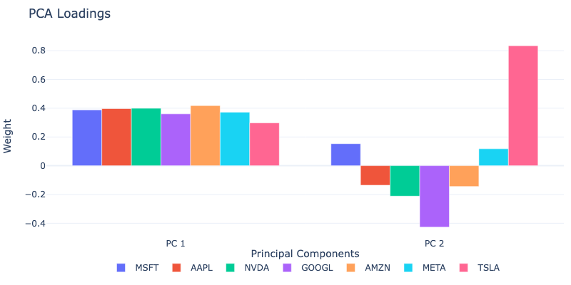
We also find that the first principal component explains roughly 62% of the total variance, as measured by the ratio of its eigenvalue to the sum of all eigenvalues. This already gives a strong signal that there is a single dominant common factor at play, and in fact we even start to see the relative weight in each sector from this, such as Technology (XLK) as the largest loading.

From Components to Portfolios

An eigenvector on its own isn’t directly investable — it’s a set of loadings, not portfolio weights, and those loadings are scale-sensitive to each asset’s volatility. Avellaneda and Lee (1) resolve this by defining an eigenportfolio: take the eigenvector loadings and normalize each by its asset’s return volatility.

\[w_i = \frac{v_i}{\sigma_i}\]

This rescaling turns the abstract “direction of maximum variance” into a concrete, tradable set of portfolio weights where each asset is weighted in proportion to how much it contributes to the common factor, adjusted for how volatile it individually is.

The Test: Does PC1 Look Like the Market?

Here’s the question we set out to answer: if the first eigenportfolio really is capturing the dominant common factor in these returns, we’d expect it to track something we’d already recognize as “the market” for instance, a broad index like the S&P 500 without ever having been told that index exists. We construct the first eigenportfolio by applying these volatility-adjusted weights to the asset returns directly. The two are shown below:

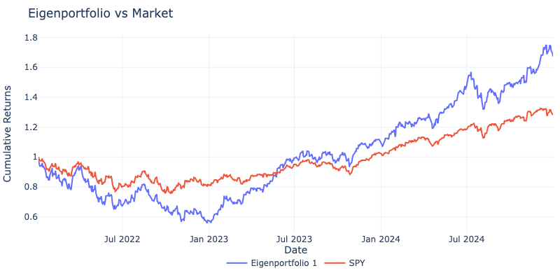
The two track each other closely. The eigenportfolio was built with no reference to the S&P 500 at all, it emerged purely from the covariance structure of a handful of industry ETFs and yet it still recovers something that looks like the market.

Why This Is Useful, Not Just Neat

It’s tempting to read this as a cute confirmation of something we already knew, of course a diversified basket’s dominant factor looks like “the market.” But the value isn’t in trading the eigenportfolio itself; it’s in what the method actually buys you.

Whenever “the market” isn’t a well-defined, off-the-shelf object such as when were dealing with a custom universe of futures, or a sector-specific basket, this approach gives you a way to construct a market-like factor directly from the data, with no external benchmark required. That’s directly useful for building hedges: if you can recover the dominant common factor statistically, you can hedge exposure to it even when there’s no natural index to short against.

We’ll leave the hedging construction for another post but the core idea stands: you don’t need to assume what the market is. You can just let the data show you.

References

• (1) Avellaneda, M., & Lee, J.-H. (2008). Statistical Arbitrage in the U.S. Equities Market. arXiv. https://arxiv.org/abs/0807.1551
• (2) Aldridge, I., & Avellaneda, M. (2021). Chapter 6. In Big Data Science in Finance. John Wiley & Sons, Incorporated.