Stylized facts of equity returns and volatility
An empirical review of stylized facts of equity returns and volatility, and their implications for modelling.
January 2025
Introduction
This post is the first the of a year-long series where I’ll be exploring various topics in quantitative finance. My goal is to publish at least twelve posts, most of which will be shared toward the end of each month.
To begin, I’ll be covering some fundamental properties- often referred to as ‘stylized facts’ of returns and volatility. The accompanying code can be found on my github profile, which is linked at the bottom of this site.
This post draws inspiration from Chapter 2 of Elements of Quantitative Investing (EQI) by Gappy, a book I’ve recently been working through. Additionally, I’ll make use of the folling references, which I highly recommend reading.
- (1) Cont, R. (2001). Empirical properties of asset returns: Stylized facts and statistical issues. Quantitative Finance, 1(2), 223-236.
- (2) Ratliff-Crain, M., Thomakos, D., Wang, T., & Xia, Y. (2022). Revisiting Cont’s stylized facts for modern stock markets. Quantitative Finance and Economics, 6(4), 568–590.
- (3) Paleologo, G. A. (2025). The Elements of Quantitative Investing. Hoboken, NJ: Wiley.
Returns
Since we’re looking the properties of returns, it’s useful to explicitly define what I use as returns. More specifically, we’ll define the return \(r(t)\) as the log return. Mathematically that is,
$$ r(t) = \log\left(\frac{P_t}{P_{t-1}}\right) = \log(P_t) - \log(P_{t-1}) $$
where:
- \(P_t\) is the price at time \(t\)
1. Lagged Auto-correlations are small.
The first property of financial returns is the small auto-correlations among log returns. Note the time scale used here is daily. The ACF plots for common equity names are given below.
Log Return ACF
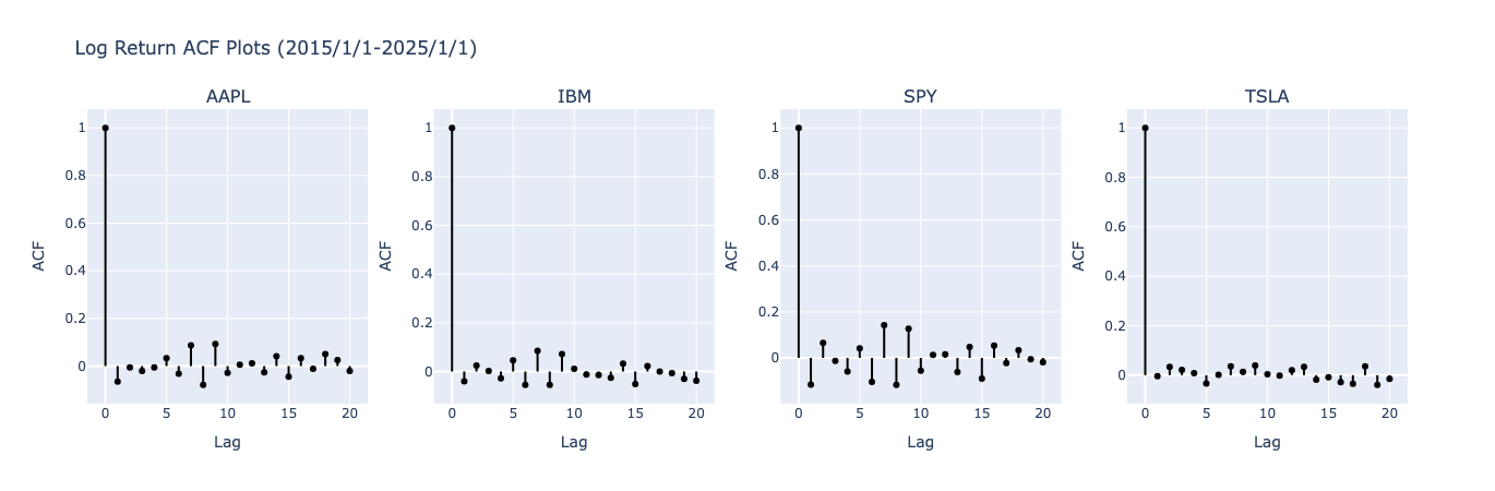
It seem fairly logical that returns have little auto-correlation among them, but this doesn’t mean returns are not predictable or independent - zero correlation does not imply independence.
2. Heavy Tails
The heavy tailed nature of returns is perhaps the most well known properties of returns, and is given as our second stylized fact. One major assumption (and/or flaw) of traditional finance models is that returns are normally distributed. We can empirically show that log returns are infact leptokurtic (they have heavier tails than a normal distribution).
To acquire estimates for the skewness and mean, I’ve applied random sampling from these emperical observations. The excess kurtosis and skewness, and confidence intervals can be seen in the table below. These values in fact do indicate a non-normal distribution with heavy tails - as seen by the excess kurtosis.
| Stock | Skew (Mean) | Skew (lower CI) | Skew (upper CI) | Kurtosis (Mean) | Kurtosis (lower CI) | Kurtosis (upper CI) |
|---|---|---|---|---|---|---|
| AAPL | -0.2 | -0.8 | 0.4 | 5.3 | 2.8 | 8.6 |
| IBM | -0.7 | -1.7 | 0.3 | 10.2 | 5.9 | 15.9 |
| SPY | -0.8 | -2.1 | 0.5 | 13.0 | 4.8 | 22.9 |
| TSLA | -0.1 | -0.6 | 0.4 | 4.4 | 2.9 | 6.2 |
3. Autocorrelations of Absolute and Square Returns
Another property of empircal return data is the high autocorrelations of absolute log returns and square log returns. The presence of autocorrelations between square returns and absolute returns can attributed to volatility clusteirng, which will be covered later. The ACF plots below should be sufficient for now to convince you of this fact, but we will make this more rigorous in a later section.
Absolute Log Returns 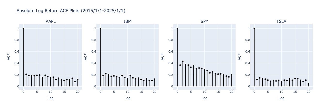
Square Log Returns 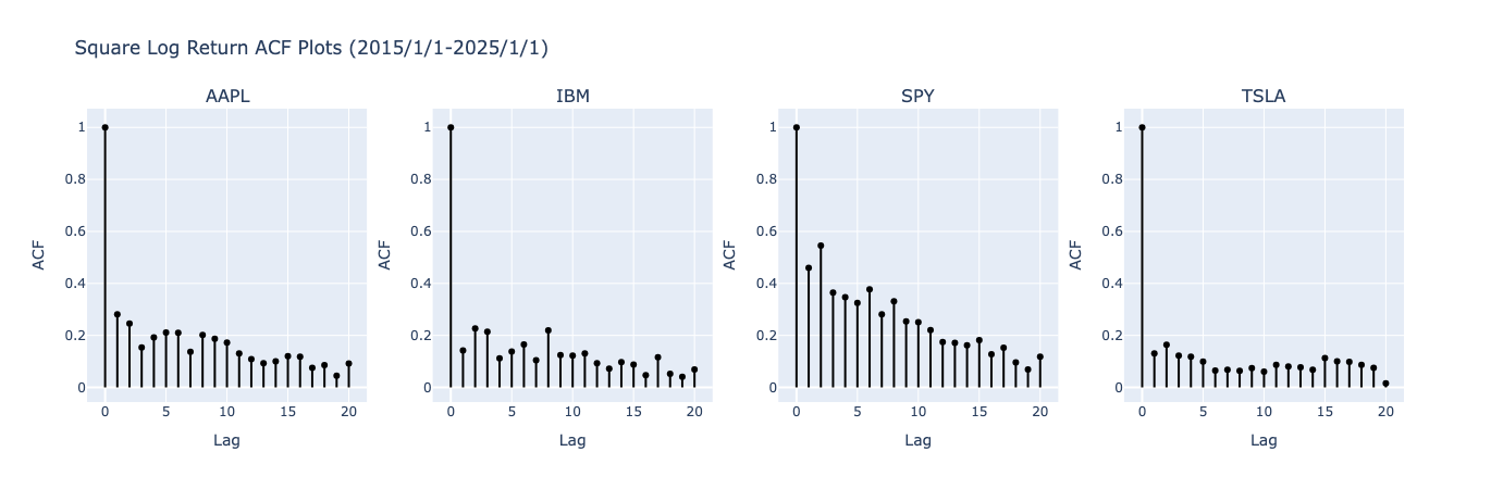
4. Aggregational Gaussinaity
Our final property of empircal returns is that when returns are calculated at longer time horizons they begin to approach normal distributions. As was pointed out in 2, daily returns do not follow strictly normal distributions given their heavy-tailed nature. When taking returns at longer horizons, however, the normal distribution might be a better approximation. In the below graph, I show the distributions of weekly, daily and monthly log returns.
Log Return Histograms 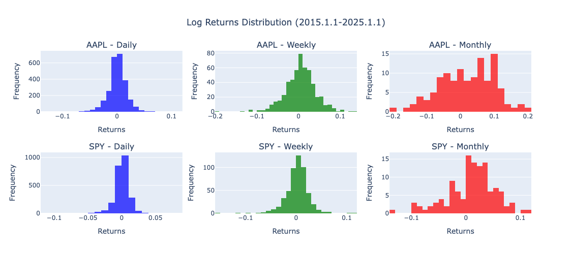
While we can see the approximate change in the histograms, we can make this more precise by applying the Kolmogorov-Smirnov Test. This statistical test allows one to compare a given distrbution to a sample. In our case, the reference distribution is the normal distribution.
The null-hypothesis of the test (in our setting) is that the data follows a normal distribution, the alternative being it does not follow a normal distribution. The results are shown in the table below, categorized by frequency and ticker.
Kolmogorov-Smirnov Test Results
| Ticker | Daily - Statistic | Daily - p-value | Weekly - Statistic | Weekly - p-value | Monthly - Statistic | Monthly - p-value |
|---|---|---|---|---|---|---|
| AAPL | 0.0773 | 0.0 | 0.0535 | 0.0968 | 0.0800 | 0.4046 |
| IBM | 0.0887 | 0.0 | 0.0781 | 0.0033 | 0.0639 | 0.6866 |
| SPY | 0.1065 | 0.0 | 0.0811 | 0.0019 | 0.1100 | 0.1013 |
| TSLA | 0.0652 | 0.0 | 0.0479 | 0.1765 | 0.0574 | 0.8021 |
Using a signifigance threshold of 0.05, we see that we’ll reject the null hypothesis for all daily return distributions, fail reject the null hypothesis for the monthly distributions and some mixed results for the weekly returns. These results both confirm that our daily returns are not normally distributed but our monthly returns are normally distribution according to this test.
Volatility
We’ll next cover a few properties of empircal volatility data, which of course goes hand in hand with the properties of returns.
1. Volatility Clustering
One of the most observable and perhaps well known empircal facts of return volatility is known as volatility clustering. This is the idea that there are periods of both high and low volatility in the market. If you’ve ever tried to fit a linear regression model to raw returns you’d notice a clear issue in your residuals as a result. We can observe this graphically by looking at the time series of return data.
Log Return Time Series
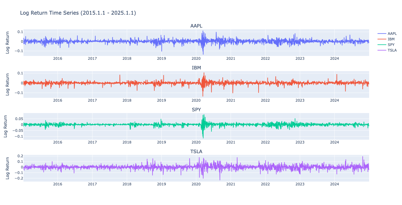
Its clear in all of the above graphs there are “clusters” of high and low volatilities. We could also see this by looking at both the absolute value or squared returns.
Squared Log Return Time Series
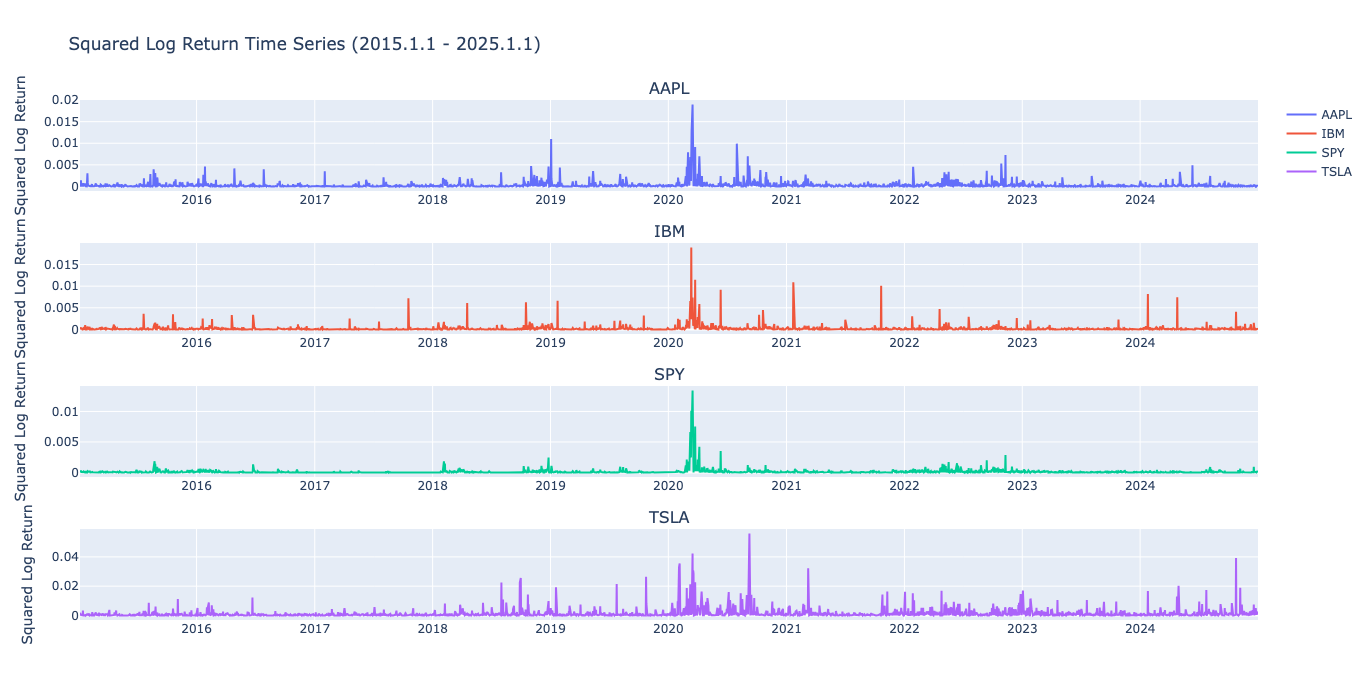
Absolute Log Return Time Series
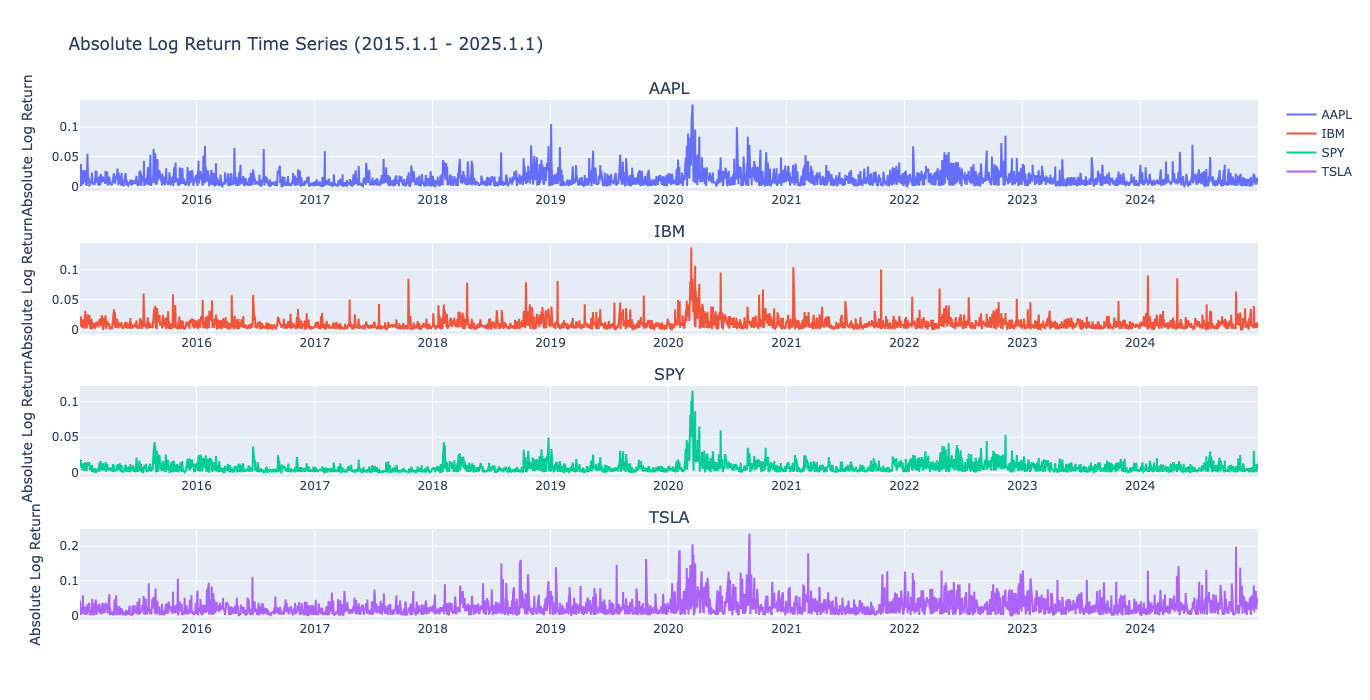
While the above plots and the autocorrelation plots that we saw in 2 of returns should hopefully convince you this property - if you’re still skeptical, lets make it more rigorous. To do this, we can look to the ARCH-LM test, which tests for the presence of heteroskedacity (non constant-variance) in time series data. The results are shown in the table below.
| Ticker | Log Returns - Statistic | Log Returns - p-value | Absolute Log Returns - Statistic | Absolute Log Returns - p-value | Squared Log Returns - Statistic | Squared Log Returns - p-value |
|---|---|---|---|---|---|---|
| AAPL | 399.5481 | 0.0 | 399.5481 | 0.0 | 425.3867 | 0.0 |
| IBM | 309.2900 | 0.0 | 309.2900 | 0.0 | 220.2913 | 0.0 |
| SPY | 962.3074 | 0.0 | 962.3074 | 0.0 | 820.3418 | 0.0 |
| TSLA | 144.7202 | 0.0 | 144.7202 | 0.0 | 80.1797 | 0.0 |
In simple words, the null hypothesis of the ARCH-LM test is that there is no heteroskedacity present, ie the time series has constant variacne. We can see across the board, using a signifigance level of 0.05, we would reject the null hypothesis. That is, our variance is not constant across the time series - due to the volatility clustering.
2. The Leverage Effect
Moving forward, another suggest fact of volatility is known as the leverage effect. This fact suggests that returns and measures of volatility are negatively correlated. To assess this, we can look at the correlations between raw returns and use lagged absolute returns as our measure of volatility.
Volatility and Return Correlations 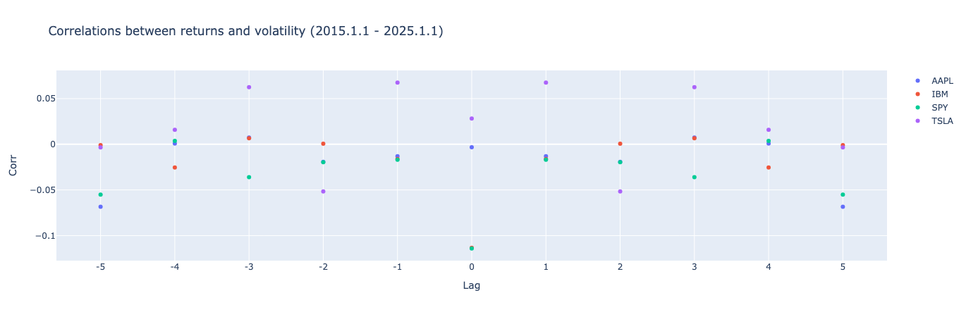
The above graph shows the correlations between returns and lagged volatility. We can see that in our sample, while some are negative, as is suggested, there are also a few positive correlations that are observable. More importantly, from a statistical point of view, these correlations are near zero and thus perhaps not meaningful. In the original paper (1), they assert that this effect is fairly strong but as we can see in our data, and the study performed in (2), they also find negilgible effect in current data.
3. Volatility and Volume
The final stylized fact of volatility that I’d like to review is the positive correlation between volatility and volume. Again, similar to how we investigated the relationship of correlations for the leverage effect, we’ll look at correlations of volume and lagged volatility (absolute log returns).
Volatility and Volume Correlations 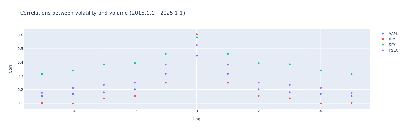
In contrast to the lack-luster results that we saw in the leverage effect, its clear there is some empircal evidence for the positive correlation between volatility and volume.
Motivation for GARCH
We covered some fairly well known properties of both returns and volatility. One might notice that many of the properties we discussed above are incredibly problematic for classical statistical models. We have non-normal distributions, possibly issues in our residuals, non-constant variance, and signifigant autocorrelations. This violates key assumptions of many linear models such as simple linear regression and simple time series models such as AR, MA or ARMA models. So what do we do?
There is of course, as given away in the title of this section a classical solution which improves the statistical properties of returns and hence makes them more susceptible to modelling. However, before we jump immediately to our solution, it’s important to provide some rational for why the GARCH model is a good choice. Sure, we could look at the results and then justify our choice, but I believe it is better to understand why the other models are not as good of a choice.
1. ARMA
First lets start with ARMA, the Autoregressive Moving-Average model. What does this model say? It says that our returns are governed by a model that contains a moving average piece and auto regressive piece. This is given by the following equation.
\[r_t = \phi_0 + \sum_{i=1}^p \phi_i r_{t-i} + \sum_{j=1}^q \theta_j \epsilon_{t-j} + \epsilon_t,\]where:
- \(r_t\) is the return at time \(t\),
- \(\phi_0\) is the intercept term,
- \(\phi_i\) are the coefficients of the AR terms (\(r_{t-i}\), lagged returns),
- \(\theta_j\) are the coefficients of the MA terms (\(\epsilon_{t-j}\), lagged error terms),
- \(\epsilon_t\) is white noise (mean zero, constant variance).
The AR terms model the dependence of \(r_t\) on its own past values, while the MA terms model the dependence of \(r_t\) on past error terms. A key assumption of this model is that it assume stationary time series and constant variance. Let’s fit model and see how this assumption breaks down.
I’ve fit an ARMA model by selecting the lowest AIC values and searching over the range of 0-4 for both p and q. Tablulated results shown here.
ARMA Models
| Ticker | Order | AIC |
|---|---|---|
| AAPL | (0, 1) | -13095.62 |
| IBM | (2, 2) | -13996.95 |
| SPY | (3, 2) | -15552.83 |
| TSLA | (2, 2) | -9599.55 |
One important issue that we should see in the residuals of the ARMA models is non-constant variance. We can clearly see this in the time series plot shown below.
ARMA Residual Time Series 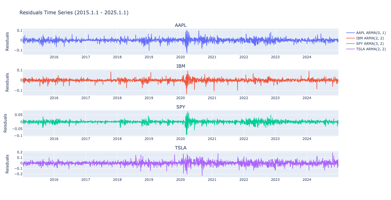
It’s not a good choice due to our volatility clusteirng.
2. ARCH
Next, let’s move on to ARCH, the Autoregressive Conditional Heteroskedasticity model. Unlike ARMA, which assumes constant variance, ARCH explicitly models the time-varying variance (volatility) of returns. The ARCH model is given by the following equations:
\[r_t = \mu + \epsilon_t, \quad \epsilon_t \sim N(0, \sigma_t^2),\] \[\sigma_t^2 = \alpha_0 + \sum_{i=1}^q \alpha_i \epsilon_{t-i}^2,\]where:
- \(r_t\) is the return at time \(t\),
- \(\mu\) is the mean return,
- \(\epsilon_t\) is the error term at time \(t\), assumed to be normally distributed with zero mean and variance \(\sigma_t^2\),
- \(\sigma_t^2\) is the conditional variance at time \(t\),
- \(\alpha_0\) is a positive constant,
- \(\alpha_i\) are the coefficients of the lagged squared error terms (\(\epsilon_{t-i}^2\), past shocks).
The key feature of ARCH is that it captures volatility clustering, where periods of high volatility are followed by high volatility, and periods of low volatility are followed by low volatility. That said, ARCH models can struggle when capturing more complex patterns of volatility. This is where GARCH models extend ARCH by including lagged conditional variance terms.
In the same manner as ARMA, I’ve fit ARCH models up to q = 4. The tablulated results and residuals, for comparison are given below.
ARCH Models
| Ticker | Order | AIC |
|---|---|---|
| AAPL | 4 | -13450.05 |
| IBM | 4 | -14268.35 |
| SPY | 4 | -16621.88 |
| TSLA | 4 | -9812.74 |
ARCH Residual Time Series 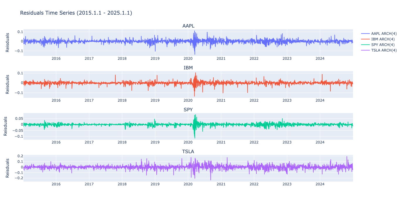
These residuals look signifigantly better than the ARMA model, and the improvement is also clear in the AIC values.
3. GARCH
Our final model, as hinted to, is the Generalized Autoregressive Conditional Heteroskedasticity model, GARCH. GARCH extends the ARCH model by incorporating lagged values of the conditional variance into the model. It is given by the following equations:
\[r_t = \mu + \epsilon_t, \quad \epsilon_t \sim N(0, \sigma_t^2),\] \[\sigma_t^2 = \alpha_0 + \sum_{i=1}^q \alpha_i \epsilon_{t-i}^2 + \sum_{j=1}^p \beta_j \sigma_{t-j}^2,\]where:
- \(r_t\) is the return at time \(t\),
- \(\mu\) is the mean return,
- \(\epsilon_t\) is the error term at time \(t\), assumed to be normally distributed with zero mean and variance \(\sigma_t^2\),
- \(\sigma_t^2\) is the conditional variance at time \(t\),
- \(\alpha_0\) is a constant (must be positive),
- \(\alpha_i\) are the coefficients of the lagged squared error terms \(\epsilon_{t-i}^2\),
- \(\beta_j\) are the coefficients of the lagged conditional variance terms \(\sigma_{t-j}^2\).
The GARCH model is more flexible than ARCH because:
- It captures volatility clustering (like ARCH),
- It accounts for the persistence of volatility through the lagged variance terms \(\sigma_{t-j}^2\).
Lets now fit a GARCH model and see how it stacks up to the previous models. Again, I’ve fit GARCH models up to p,q = 4. The orders and AIC values for the best models are given below, alongside the residual time series.
GARCH Models
| Ticker | Order | AIC |
|---|---|---|
| AAPL | (1, 2) | -13576.29 |
| IBM | (1, 1) | -14303.41 |
| SPY | (1, 1) | -16692.52 |
| TSLA | (1, 1) | -9928.35 |
GARCH Residual Time Series 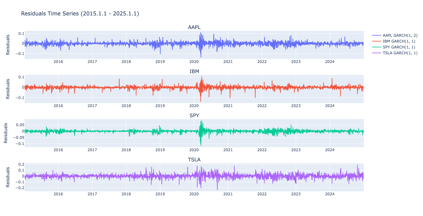
Improvemens from GARCH
It’s perhaps clear from the AIC values that both ARCH and GARCH models provide an improvement over models traditional time series models such as ARMA, but there are further reasons aside from the ‘fit’ that one should consider GARCH. Specifically, modelling the returns as a GARCH process address many of the return stylized facts that we outlined above, such as the absence of autocorrelations, heavy tailedness, autocorrelations of squared and absolute returns, and aggregation gaussinatity. For further mathematical reasoning behind these properties I defer to EQI Chapter 2.
Conclusion
In this post, we provided a brief overview of the key properties of financial returns and volatility and the implications these properties have for modeling. We also discussed the motivation behind using classical models like GARCH to capture these dynamics effectively. Hopefully, by understanding these foundational concepts, we gain an understanding that will guide as a we move into more advanced analysis.
Stay tuned for future posts in this series, where I’ll continue to explore topics in quantitative finance. As always, you can find additional resources and code on my GitHub. Thank you for reading!