Selecting suitable projection matrices for compressed NMF

Introduction

In this post, I provide a breif summary of a research project I recently completed as part of STAT6104 - Computational Statistics at Columbia. The goal of the course and project, was as the name suggests, to explore computational techniques which improve the ability to apply statistical algorithms to large scale data. If you’re interested, you can access my full paper, slides from my presentation and all code here.

A review of NMF

NMF, originally proposed by Lee in Seung in 2000, has become a popular matrix factorization technique and is commonly viewed as an alternative to Principal Component Analysis (PCA). In contrast to PCA, however, as the name suggests, NMF generates strictly non-negative components. This aspect is important for fields in which negative factor weights do not hold meaningful interpretations, such as with text data. We formalize the problem below.

The problem statement

Given a non-negative data matrix \(A \in \mathbb{R}^{m \times n}_{\geq 0}\), NMF seeks factor matrices \(W \in \mathbb{R}^{m \times k}_{\geq 0}\) (basis) and \(H \in \mathbb{R}^{k \times n}_{\geq 0}\) (coefficients) with \(k \ll \min(m,n)\) such that:

\[X \approx WH,\]

where the approximation minimizes \(\|A - WH\|_F^2\) subject to the non-negativity constraints \(W_{ij}, H_{ij} \geq 0 \ \forall i,j\)

Given that the problem itself is both non-convex and NP hard in general, iterative solutions are required. The most common of these is the multiplicative update rule, also introduced by Lee and Seung. In these updates, for each iteration one matrix is held fixed while the other is updated. They are given as follows:

\[\begin{align} W &\leftarrow W \otimes \frac{AH^T}{WHH^T} & H &\leftarrow H \otimes \frac{W^TA}{W^TWH} \end{align}\]

While these rules are simple to implement, they suffer from increasingly high computational cost as the dimension of \(A\) grows. More specifically, each iteration requires computing a product which includes the original matrix \(A\), and that costs \(\mathcal{O}(mnk)\). This led to the natural extension of resorting to randomized linear algebra techinques such as randomized projections.

Compressed Methods

As motivated earlier, we now explore two extensions of the original NMF algorithms that use randomized projections to achieve equivalent factorizations at significantly lower computational cost. Randomized projection is based on the Johnson-Lindenstrauss lemma, which guarantees that pairwise distances can be preserved when projecting to a lower-dimensional space. This is commonly implemented by left-multiplying the input matrix by a random projection matrix, which we denote as \(\Omega\).

1. Compressed NMF

The compressed NMF approach accelerates computation by first reducing the dimensionality of the input matrix through randomized projections. For a given non-negative data matrix \(A \in \mathbb{R}^{m \times n}\), we generate two random projection matrices: \(\Omega_m \in \mathbb{R}^{r \times m}\) for row compression and \(\Omega_n \in \mathbb{R}^{r \times n}\) for column compression, where the target dimension \(r \ll \min(m,n)\). The python implementation of the compressed algorithm is given below.

import numpy as np
def compressed_mu(X, k, r, max_iter=100):
    # Initialize random projection matrices
    Omega_m = np.random.randn(r, X.shape[0])  
    Omega_n = np.random.randn(r, X.shape[1])  
    
    # Compute compressed matrices
    X_m = Omega_m @ X  
    X_n = X @ Omega_n.T  
    
    # Initialize factors
    W = np.abs(np.random.randn(X.shape[0], k))
    H = np.abs(np.random.randn(k, X.shape[1]))
    
    for _ in range(max_iter):
        # Project current factors
        W_proj = Omega_m @ W  
        H_proj = Omega_n @ H
        
        # Update H
        H *= (W_proj.T @ X_m) / (W_proj.T @ W_proj @ H)
        
        # Update W
        W *= (X_n @ H_proj.T) / (W @ H_proj @ H_proj.T)
    
    return W, H

The result of this is reducing the computational complexity to \(\mathcal{O}(rnk + rmk)\) per iteration.

2. Structured Compressed NMF

Structured compressed NMF enhances the basic compression approach by using randomized power iteration to better preserve the dominant singular subspaces of the input matrix. This method is particularly effective when the data matrix has rapidly decaying singular values.

The randomized subspace iteration is shown in python below

def randomized_subspace_iteration(X, Omega, l, q=2):
    # Omega: projection matrix, l: target dimension, q: power iterations, 
    Y = X @ Omega
    for _ in range(q):
        Y = X @ (X.T @ Y)  # Power iteration
    Q, _ = np.linalg.qr(Y)  # Orthonormal basis
    return Q

The modification to the NMF algorithm given in compressed version is now simply to replace \(\Omega_m\) and \(\Omega_n\) with \(Q_m\) and \(Q_n\), obtained from the algorithm above.

Suitable Projection Matrices

Given the heavy reliance on projection matrices in both algorithms, my research focused on examining the impact of different projection matrix choices. While most implementations use Gaussian random matrices, these can be undesirable for sparse data as they could both destroy sparsity and increase computational costs. I evaluated four alternative projection matrix types:

Projection Type	Construction	Sparsity	Complexity	Key Property
Gaussian	\(\Omega_{ij} \sim \mathcal{N}(0,1)\)	Dense	\(\mathcal{O}(mnr)\)	Optimal JL guarantees
SRHT	\(SHD\) (Hadamard + Rademacher)	Dense	\(\mathcal{O}(mn\log r)\)	Fast transform
SRFT	\(SFD\) (Fourier + Rademacher)	Dense	\(\mathcal{O}(mn\log r)\)	Non-uniform FFT
CountSketch	One \(\pm 1\) non-zero per column	Sparse	\(\mathcal{O}(\text{nnz}(X))\)	Streaming-friendly
Sparse JL	\(s=1\) non-zero per column	Sparse	\(\mathcal{O}(s\cdot\text{nnz}(X))\)	Better variance

Performance

Finally, to evaluate the practical trade-offs between computational efficiency and reconstruction quality, I tested each algorithm-projection matrix combination on both synthetic and real-world data. Synthetic matrices were generated with controlled density (\(\delta = 1.0\) for dense, \(\delta = 0.01\) for sparse cases) using the low-rank ground truth methodology from the paper. For empirical validation, I focused on the Olivetti Faces dataset, which is a dense 400×4096 matrix of 64×64 pixel facial images, where visual reconstruction quality provides intuitive assessment of the factorization. All implementations were standardized at 100 iterations, fixed random seeds and evaluated on both runtime and relative Frobenius norm error \(\|X-WH\|_F/\|X\|_F\). While the full paper includes additional analysis of sparse text data, here I only show the application to the dense case.

Synthetic

A more in depth analysis of the computational cost reduction for compressed methods is given in the full paper. Here, we review broader results for the full NMF computation, shown in the Figures below. Note that inlucded in the below plots is also the performance of an additional algorithm known as Hiearchical Alternating Least Squares (HALS).

Synthetic Dense Matrices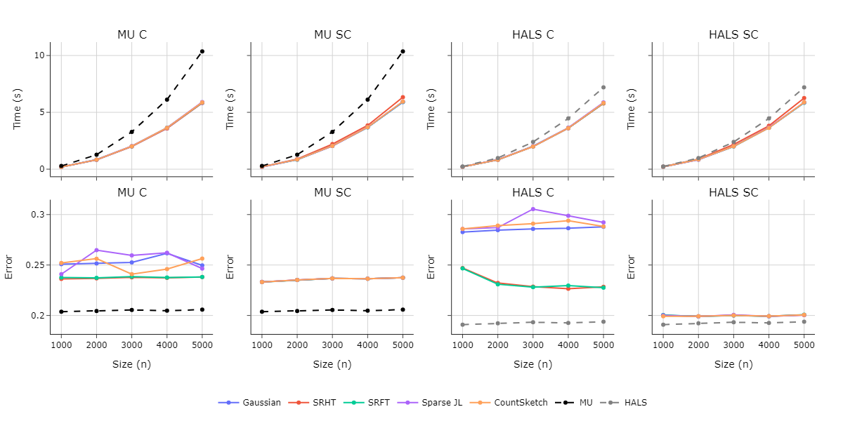

Synthetic Sparse Matrices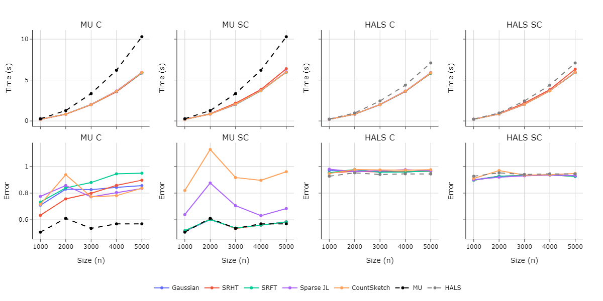

The results demonstrate that compressed and structured compressed NMF algorithms consistently outperform traditional NMF approaches, with performance varying according to both projection matrix selection and input matrix density. For dense matrices, we show that HALS C achieves the best performance when combined with SRFT or CountSketch projections, yielding significant improvements in reconstruction accuracy without compromising computational efficiency. In the case of sparse matrices, MU SC proves most effective when paired with SRFT, Gaussian, or SRHT projections, similarly balancing error reduction with computational performance. These findings highlight the importance of selecting projection matrices that are appropriately matched to both the matrix density and algorithm type, suggesting that practitioners should carefully consider these relationships when implementing compressed NMF methods. The observed variability in performance across different projection matrices also reinforces that optimal configurations are context-dependent, with each projection type offering distinct advantages for particular combinations of input characteristics and algorithmic approaches.

Empirical (Olivetti Faces)

Finally, we explore Olivetti Faces Database, a standard benchmark for matrix factorization methods. The dataset comprises \(400\) grayscale facial images (\(64 \times 64\) pixels) from \(40\) subjects, yielding a dense \(400 \times 4096\) matrix with \(0.01\%\) sparsity.

For all experiments, we fix the reduced rank at \(r = 49\) for the factor matrices \(W\) and \(H\). Further, to account for the inherent randomness in both the compression steps and initialization, we report mean reconstruction errors (computed as \(\|{X} - WH^\top\|_F/ \|X\|_F\)) and computation times averaged over 10 independent trials (implemented as different seeds). These results are summarized in the table below.

\[\begin{array}{lcccccc} & \text{HALS C} & \text{HALS SC} & \text{MU C} & \text{MU SC} & \text{HALS} & \text{MU} \\ \hline \textbf{Errors} \\ \hline \text{None} & - & - & - & - & 0.1508 & 0.1381 \\ \text{Count-Sketch} & 0.1800 & 0.1492 & 0.1881 & 0.1808 & - & - \\ \text{Gaussian} & 0.1738 & 0.1492 & 0.1901 & 0.1808 & - & - \\ \text{Sparse-JL} & 0.1753 & 0.1495 & 0.1858 & 0.1808 & - & - \\ \text{SRFT} & 0.2037 & 0.1492 & 0.2258 & 0.1808 & - & - \\ \text{SRHT} & 0.1966 & 0.1491 & 0.2254 & 0.1809 & - & - \\ \hline \textbf{Time (s)} \\ \hline \text{None} & - & - & - & - & 0.7604 & 0.9024 \\ \text{Count-Sketch} & 0.5449 & 0.5642 & 0.4117 & 0.5360 & - & - \\ \text{Gaussian} & 0.5329 & 0.5790 & 0.4345 & 0.4707 & - & - \\ \text{Sparse-JL} & 0.5486 & 0.5914 & 0.4301 & 0.5113 & - & - \\ \text{SRFT} & 0.5391 & 0.5700 & 0.4495 & 0.5028 & - & - \\ \text{SRHT} & 0.5588 & 0.5920 & 0.4301 & 0.5038 & - & - \\ \end{array}\]

The experimental results confirm that compressed algorithms universally reduce computational time compared to their uncompressed counterparts, regardless of update rule or projection matrix choices. While this acceleration introduces marginally higher reconstruction errors, these remain within acceptable tolerances for practical applications. In particular, the projection matrix selection proves consequential for compressed algorithms, with errors approaching those of their structured compression counterparts. For example, Gaussian projections optimize performance for HALS C, while Sparse-JL achieves superior results for MU C. Moreover, given the similarity in reconstruction errors across MU SC and HALS SC algorithms, one might simply choose the one with faster computation time (CountSketch and Gaussian respectively). These findings demonstrate that while compression necessarily involves speed-accuracy trade-offs, informed algorithm-matrix pairings can effectively balance these competing priorities, with optimal configurations being method dependent. Finally, the figures below showcase sample reconstructions using optimal projections obtained from the table above.

MU Reconstruction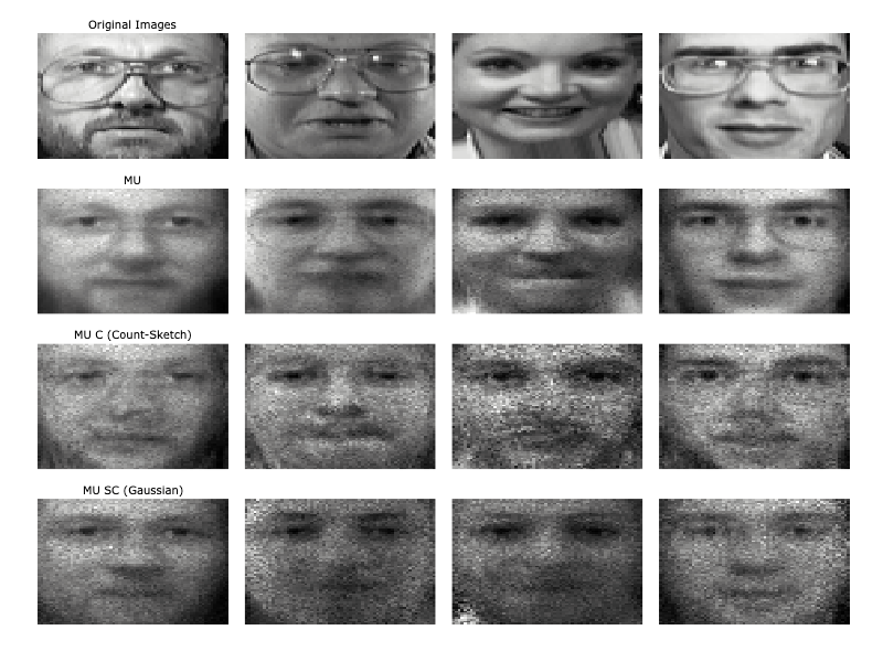

Conclusion

In this research, we investigated the use of non-Gaussian projection matrices within compressed and structured compressed NMF algorithms. We conducted numerical experiments on synthetic dense and sparse datasets, then empirically examined the impact of projection matrix selection on reconstruction error and runtime. Our results show that, under certain conditions, an appropriate choice of projection matrix can reduce computational cost without increasing reconstruction error or reduce reconstruction error without increased computational cost.

Again for a more in depth version of my research project, please read the full paper linked at the top of this post. Thanks for reading!