The game of 24 - a short analysis and some strategies

Before moving to New York and starting grad school, I hadn’t spent much time using subway systems, my commute during undergrad in Montreal was a mere 15 minute walk. In New York, I wasn’t as lucky (relatively speaking, on a commute basis) - so I found myself spending a significant amount of time in the subway system, where cellular service is spotty at best. Sure – there’s a bunch of things I could do, read papers, read a book, listen to music but after a long day in classes those seem to draining so I’d often opt for some type of game on my phone. One big downside is a lot of games require internet service, so I needed to find one that was sufficiently interesting, required no cell service, and ideally keep me entertained for at least a few weeks until I moved onto another.

The Game of 24

Eventually I came across what I’ll refer to as “The Game of 24”. It’s fairly simple and perhaps boring to those who are uninterested testing/improving their simple arithmetic.

The game is as follows. You’re given 4 numbers and you need to apply operations to these numbers; addition, subtraction, multiplication or division, such that the end result is 24. For example, if you’re given 4,6,2,1. You could input:

\[4 \times 6 \times (2-1) = 24 \times 1 = 24.\]

That’s it. That’s all there is to the game. So why are you reading this, and why am I writing it? The game itself has 1200 levels total, 400 “easy”, 400 “medium” levels, 400 “hard” levels. However, in my experience, 800/1200 levels completed so far, the difficulty is not always commensurate with the amount of time it takes me to solve them, with most taking me <5 seconds or much longer depending on my energy levels.

Either way, I’ve had a few questions in mind that I’d like to answer, which serve two main purposes for me. The first, how many more levels could I solve – 1200 seems arbitrary and is surely not the limit but just a round number the developer stopped at. The second, how can I improve my current strategy to solve questions faster. Here’s a list of the main questions I’m hoping to answer throughout this post, which should help me with the above.

• How can I quantify easy, medium and hard questions? How many of each type are there?
• Which numbers often pair together, and how could I recognize that fast? For example, 6x4 or 8x3 appear fairly often.
• Which numbers quadruples have the most solutions?

Enumerating All Solutions

Let’s first note that, in the way the current game was developed, the same number can appear multiple times in your board. For example, 4,4,8,1 is a valid starting board and indeed has a solution (find it).

A natural first step is to ask how many boards we can create? This itself is a fairly simple counting exercise; we have 12 choices for each number, and to create each solution, we need to choose 3 operators, from a selection of 4. This leads us to

\[12 \times 4 \times 12 \times 4 \times 12 \times 4 \times 12 = 12^4 \times 4^4\]

possible combinations.

Is that it? No, order of operations matters, so we need to also place parentheses. It’s not difficult to reason, there’s 5 ways to place these parentheses. So we end up with

\[5 \times 12^4 \times 4^4 = 6,635,520\]

possible ways to add, subtract, multiply and divide 4 numbers to arrive at some result. Of course, not all of these are equal to 24.

Okay, enough thinking, let’s write some simple Python code to generate all of these combinations, and the verify which of those correctly equate to 24.

nums = list(range(1, 12 + 1))
ops = ['+', '-', '*', '/']

def evaluate_expression(expression):
    try:
        return eval(expression) == 24
    except ZeroDivisionError:
        return False

valid = set()
counts = defaultdict(list)
i = 0
# Generate all permutations of 4 numbers
for num_perm in product(nums, repeat=4):
    num1, num2, num3, num4 = num_perm
    # Generate all combinations of 3 operators
    for op_comb in product(ops, repeat=3):
        op1, op2, op3 = op_comb
        # Different ways to parenthesize expressions
        expressions = [
            f"({num1} {op1} {num2}) {op2} ({num3} {op3} {num4})",
            f"(({num1} {op1} {num2}) {op2} {num3}) {op3} {num4}",
            f"({num1} {op1} ({num2} {op2} {num3})) {op3} {num4}",
            f"{num1} {op1} (({num2} {op2} {num3}) {op3} {num4})",
            f"{num1} {op1} ({num2} {op2} ({num3} {op3} {num4}))"
        ]
        # Evaluate each expression
        for expr in expressions:
            i += 1
            if evaluate_expression(expr):
                valid.add(expr)
                counts[','.join([str(x) for x in sorted(num_perm)])].append(expr)

The result is: 41,818 number of possible solutions to our game. Now, you also might have thought, some of these use the same combination of numbers - so let’s group them by the numbers they use. The below shows the groupings with the most amount of possible solutions.

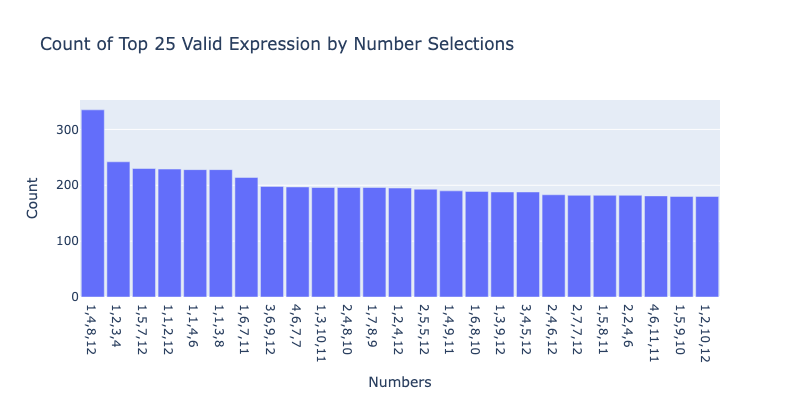
Now let’s look at the distribution of number of solutions.

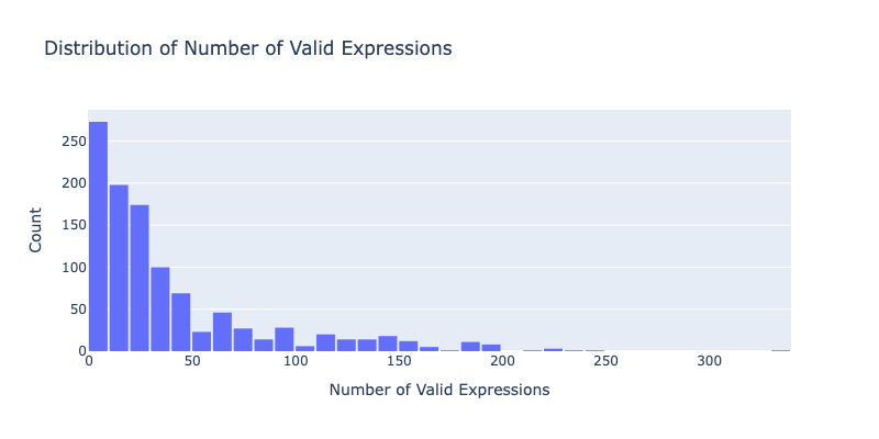
Classifying Difficulty

Now, let’s try to define what an easy, medium, or hard problem is. In my opinion, and what I feel is most logical – the difficulty of the problem should be related to the number of possible solutions, so we will use this as our only feature.

Thresholding

Perhaps the first logical approach, and maybe the one that was used in creation of the game was simply to group problems by the number of solutions. For example, we could consider all of the problems with 20 solutions to be difficult, while those with between 20 and 40 solutions “medium”, and anything beyond that as easy.

If we used this rule, the count of easy, medium and hard problems would be as follows.

\[\begin{array}{l r} \textbf{Difficulty} & \textbf{Count} \\ \hline \text{Easy} & 311 \\ \text{Medium} & 233 \\ \text{Hard} & 524 \end{array}\]

Mixture Models

Model overview

Now, since our goal was to label the problems as easy, medium, or hard, we could perform an unsupervised learning method known as mixture-modeling. The general idea is that each problem’s number of solutions is generated from a combination of underlying distributions corresponding to the difficulty levels. Formally, a mixture model can be written as:

\[p(x_i) = \sum_{k=1}^{K} \pi_k \, f_k(x_i \mid \theta_k)\]

where:

• \(K\) is the number of components (here, the difficulty levels),
• \(\pi_k\) is the proportion of problems in component \(k\) (so that \(\sum_k \pi_k = 1\)),
• \(f_k(x_i \mid \theta_k)\) is the probability distribution for component \(k\), parameterized by \(\theta_k\),
• and each \(x_i\) (the number of solutions for problem \(i\)) is drawn independently from this mixture.

For count data like the number of solutions, the \(f_k\) might be a Poisson, negative binomial, or log-normal distribution. Then once the mixture model is fitted, each problem can be assigned to a cluster probabilistically, giving us soft labels for easy, medium, or hard.

Model specification

For this data I’ve chosen to fit a Poisson-Lognormal Mixture model, which can be described via the following model:

\[x_i \sim \sum_{k=1}^{K} \pi_k \, \text{Poisson}(\lambda_i), \quad \lambda_i \sim \text{LogNormal}(\mu_k, \sigma_k^2)\]

with:

• \(K = 3\) mixture components
• \(\lambda_i\) is the latent Poisson rate for problem \(i\), drawn from a log-normal distribution with parameters \(\mu_k\) and \(\sigma_k^2\) specific to component \(k\),
• and \(x_i\) is the observed number of solutions for problem \(i\).

In this setup, each cluster represents a difficulty level, and the Poisson-Lognormal mixture allows us to capture both the discrete nature of solution counts and the heavy-tailed variability across problems. I’ll skip most the implementation details, but they are available [here].

Results

First, the graph. The graph below shows the re-labeled distribution of our problem solutions according to their difficulty level as output by our Poisson-Lognormal mixture model. Problems with fewer solutions are labeled as Hard, those with medium counts as Medium, and those with many solutions as Easy.

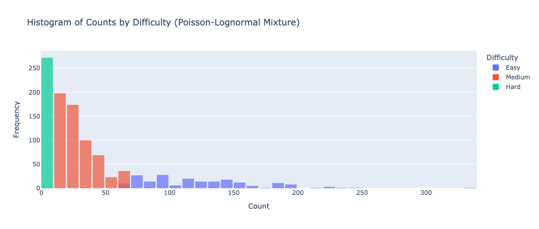
Further, summary statistics for these categories are shown in the following table:

\[\begin{array}{l r r} \textbf{Difficulty} & \textbf{Num. Problems} & \textbf{Median Num. Solutions} \\ \hline \text{Easy} & 195 & 114.0 \\ \text{Medium} & 601 & 24.0 \\ \text{Hard} & 272 & 4.0 \end{array}\]

Analysis & Strategies

Okay, now that we have some sense of what difficulty level of problems are available, I also wanted to find some additional strategies (from the data) that could help me solve these faster.

Common Operations

Lets first start by identifying the most common operation in the solutions.

\[\begin{array}{l r} \textbf{Operator} & \textbf{Count} \\ \hline \times & 35{,}499 \\ \div & 16{,}466 \\ + & 48{,}078 \\ - & 25{,}411 \\ \end{array}\]

From the data, we can see that addition and multiplication are the most frequent operations, followed by subtraction and division. This suggests that focusing on these common operations could help solve problems more efficiently.

First operation pairs

The table below shows the most common first operations in problem solutions. Looking at these patterns, we can see which number pairings and operations are used most often, giving insight into strategies that might help solve similar problems faster.

As expected, factors of 24 dominate the top of the list, which reinforces that spotting direct factors of 24 or 12 early is a common and useful strategy.

Operation	Count
2 * 12	201
3 * 8	201
4 * 6	201
12 + 12	201
6 + 6	149
11 + 1	149
8 + 4	149

Takeaways

So what’s the takeaway? Clearly, the game’s creator didn’t put nearly as much thought into difficulty categorization as I did here — which explains why some of the problems labeled easy actually felt hard. On the bright side, this analysis has given me some data-driven strategies to rely on when I get stuck, making it easier to approach those tricky problems.