Statistical factor models, and factor discovery

Introduction

It’s April- and this is another one of my monthly posts. To catch up on the others, please visit the monthly folder here.

Today were going to examine different ways of generating factors to be used within a statistical factor model, such as using PCA, SPCA and IPCA. Importantly, the content of this post will be somewhat self contained, however, it does have close ties to a few topics that I have already covered in previous posts, such as eigenportfolios see this here, or a brief introduction to factor models given in this post here.

Towards Statistical Factor Models

Fundamental and Macroeconomic Factor Models

First, lets define what a factor model is. A factor postulates that returns are driven by a few “random” factors in the market. In mathematical terms we write:

\[r_t = \alpha + Bf_t + \epsilon_t\]

where \(r_t \in \mathcal{R}^{n \times 1}\) is our random vector of returns at time \(t\), \(B \in \mathcal{R}^{n \times m}\) loadings matrix, \(f_t \in \mathcal{R}^{m \times 1}\) is our factor returns at time \(t\), and finally \(\epsilon_t \in \mathcal{R}^{n \times 1}\) is our idiosyncratic returns. Importantly, there are two types of factor models of the form given above. The first of which, is the fundamental factor model, in this model we assume that we are given the loadings matrix \(B\) and then we must estimate \(f_t\) and \(\epsilon_t\). The second type of model is the macroeconomic factor model, where we have the reverse problem. We select some set of factors for which we have a return series, for example the fama-french model, and then we estimate \(B\) (time-series regression).

Statistical Factor Models

The statistical factor model is the natural extension to the above formulation, however, now we assume that we know neither both \(F\) nor \(B\). We formalize this mathematically with:

\[R \approx BF\]

where \(R \in \mathcal{R}^{n\times T}\) is our return series, \(B \in \mathcal{R}^{n \times m}\) is our loadings matrix and \(F \in \mathcal{R}^{m \times T}\) is our factor score matrix.

Estimating Statistical Factor Models

A first approach

As a first step towards estimating the statistical factor model, one might consider solving the following problem:

\[\underset{B,F}{\min} \| R - BF \|_F\]

For many, this problem should seem familiar. We can just perform a singular value decomposition on the matrix \(R\), to obtain \(U\), \(S\) and \(V\) where \(R = USV^\top\). Then if we wanted to recover our matrices \(B\) and \(F\), simply let

\[\begin{align} B & = U \\ F & = S V^\top \end{align}\]

Given a return matrix \(R \in \mathcal{R}^{n \times T}\), this is easily computed in python as follows:

import numpy as np
# Given: R (n x T)
U, S, Vt = np.linalg.svd(R, full_matrices=False)
# Construct B and F
B = U
F = np.diag(S) @ Vt

We now show a nice connection between the above problem and PCA. For many, perhaps another commmon approach would be first to select the first \(m\) principal components and use these as the factor loadings. That is we let \(B = U_m\), where \(U_m\) is the first \(m\) columns of \(U\) (from SVD). Then, since we have our factor loadings, we would want to estimate \(F\). A reminder the factor model is given as:

\[\begin{align} R & = BF + E \\ & = U_m F + E \end{align}\]

We could estimate \(F\) using cross-sectional regressions, for which the least squares estimator is given as

\[\begin{align} \hat{F} & = (B^\top B)^{-1} B^\top R \\ & = (U_m^\top U_m)^{-1} U_m^\top R \\ \end{align}\]

However, since \(U\) is orthonormal by construction and we previously had \(R = U S V^\top\), then we have that

\[\begin{align} \hat{F} & = (U_m^\top U_m)^{-1} U_m^\top R \\ & = U_m^\top R \\ & = U_m^\top USV^\top \\ & = S_m V_m^\top \end{align}\]

That is, we recover the same \(B\) and \(F\) as when we had directly applied SVD to \(R\).

Two-Step PCA

The above approach is unsatisfactory for many reasons, first and foremost, we would like to have an estimate of our factor model for each \(t\). In this section, we’ll restate and provide partial motivation for the two-step PCA procedure provided in EQI Section 7.5.2 (ref. below).

First, we state the goal of this procedure, that is we want to obtain the loadings matrix \(B_t\) at every time \(t\). Then, we want to obtain an estimate of the factor returns \(f_t\) and idiosyncratic returns \(\epsilon_t\) at every time \(t\). The output of the procedure will be \(B_t\), and we can estimate \(f_t\) with time-series cross-sectional weighted regressions as we previously motivated. I provide the procedure below, with notes throughout each step.

1. Inputs

Let \(R \in \mathbb{R}^{n \times T}\). First, we choose our parameters:

\[\tau_s \geq \tau_f > 0, \quad p \in \mathbb{N}, \quad m > 0\]

In this, \(\tau_f\) and \(\tau_s\) are our decay times to be used in the first and second stage PCA respectively, \(p\) is the number of intermediate factors, and \(m\) is the final number of desired factors in the output.

---

2. Time-Series Reweighting

In the first computational step, we perform a time-sereis reweighting of our returns according to our chosen decay factor \(\tau_f\). Here \(\kappa\) is a constant which normalizes the sum of the weights to 1.

\[W_{\tau_f} := \kappa \cdot \mathrm{diag}(e^{-T/\tau_f}, \dots, e^{-1/\tau_f})\] \[\widetilde{R} = R W_{\tau_f}\]

---

3. First-Stage PCA

Now, we perform a Singular Value Decomposition on \(\widetilde{R}\). The goal here is to denoise the return matrix by identifying and removing the dominant low-rank structure (common variation) before estimating idiosyncratic volatility.

\[\widetilde{R} = \widetilde{U} \widetilde{S} \widetilde{V}^\top\]

---

4. Idiosyncratic Proxy Estimation

Then, we utilize the truncated reconstruction of \(\widetilde{R}\) to estimate the idiosyncratic volatilities.

Truncated reconstruction of rank \(p\):

\[E = \widetilde{R} - \widetilde{U}_p \widetilde{S}_p \widetilde{V}_p^\top\]

Idiosyncratic volatilities:

\[\sigma_i^2 = \frac{1}{T} \sum_{t=1}^T E_{i,t}^2\]

---

5. Idiosyncratic Reweighting

Again, before performing our second-stage PCA, we perform a time-series reweighting of the idiosyncratic volatilities. In this, we utilize \(\tau_s\) as our decay factor, and as before \(\kappa\) is a normalizing constant.

\[W_\sigma := \mathrm{diag}(\sigma_1^{-1}, \dots, \sigma_n^{-1})\] \[W_{\tau_s} := \kappa \cdot \mathrm{diag}(e^{-T/\tau_s}, \dots, e^{-1/\tau_s})\] \[\widehat{R} := W_\sigma R W_{\tau_s}\]

---

6. Second-Stage PCA

Finally, we can move onto second-stage PCA where we compute the final factor loadings \(\mathbf{B}\) and factor scores \(\mathbf{f}_t\) from a version of the return matrix where idiosyncratic noise has been minimized and recent data is emphasized (\(\widehat{R}\)).

\[\widehat{R} = \widehat{U} \widehat{S} \widehat{V}^\top\]

---

7. Factor Model Specification

Then, as we had pre-specified the desired number of final components in our model we take top \(m\) components:

\[\widehat{r} = \widehat{U}_m f + \widehat{\varepsilon}\]

---

8. Output Final Factor Model

The final output of our model is then given as:

\[B := W_\sigma^{-1} \widehat{U}_m\] \[r = B f + \varepsilon\]

so that we have

\[\hat{f} = \widehat{U}_m W_{\sigma} r \quad \text{and} \quad \hat{\epsilon} = r - B\hat{f}\]

I now provide below the Python implementation of the above procedure.

def statistical_factor_model(R, tau_s, tau_f, p, m):
    """
    Estimate a statistical factor model with time-series reweighting and two-stage SVD.
    
    Args:
        R (np.ndarray): Asset returns matrix (n x T).
        tau_s (float): Idiosyncratic reweighting decay parameter (tau_s).
        tau_f (float): First-stage decay parameter (tau_f).
        p (int): Number of factors in first-stage SVD.
        m (int): Number of factors in final model.
    
    Returns:
        B (np.ndarray): Factor loadings (n x m).
        F (np.ndarray): Factor scores (m x T).
        sigma (np.ndarray): Idiosyncratic volatilities (n x 1).
    """
    # 1. Input validation
    assert tau_s >= tau_f > 0
    n, T = R.shape
    
    # 2. First-stage reweighting
    weights_tau_f = np.exp(-np.arange(T, 0, -1) / tau_f)
    weights_tau_f *= T / np.sum(weights_tau_f)
    W_tau_f = np.diag(weights_tau_f)
    R_tilde = R @ W_tau_f

    # 3. First-stage PCA
    U_tilde, S_tilde, Vt_tilde = np.linalg.svd(R_tilde, full_matrices=False)
    U_p = U_tilde[:, :p]
    S_p = np.diag(S_tilde[:p])
    V_p = Vt_tilde[:p, :]
    
    # 4. Idiosyncratic proxy estimation
    E = R_tilde - U_p @ S_p @ V_p
    sigma_sq = np.mean(E**2, axis=1)
    sigma = np.sqrt(sigma_sq)
    W_sigma = np.diag(1 / sigma)
    
    # 5. Idiosyncratic reweighting
    weights_tau_s = np.exp(-np.arange(T, 0, -1) / tau_s)
    weights_tau_s *= T / np.sum(weights_tau_s)
    W_tau_s = np.diag(weights_tau_s)
    R_hat = W_sigma @ R @ W_tau_s
    
    # 6. Second-stage PCA
    U_hat, S_hat, Vt_hat = np.linalg.svd(R_hat, full_matrices=False)
    
    # 7. Extract top m factors
    U_m = U_hat[:, :m]
    S_m = np.diag(S_hat[:m])
    V_m = Vt_hat[:m, :]
    
    # 8. Compute outputs
    B = np.linalg.inv(W_sigma) @ U_m
    B /= np.linalg.norm(B, axis=0) 
    
    return B,W_sigma

Factor Discovery

In the above implementation, we note that the factors are discovered in the second-stage PCA via SVD. This is of course, not the only way in which we can discover factors. Two other common variants of PCA, which we now explore for factor discovery, are Sparse PCA (SPCA) and Independent PCA (IPCA). We first provide a review of both problems.

Sparse PCA

Sparse PCA, is as it sounds, it introduces sparsity in the principal components, while retaining the standard properties of PCA (orthogonal components, variance maximization etc.). Sparse PCA is formalized by including an L1 regularization term in the PCA problem. We state this mathematically below:

\[\min_{W, H} \quad \frac{1}{2} \| X - WH \|_F^2 + \alpha \sum_{j=1}^{k} \| w_j \|_1 \quad \text{subject to } \forall j: \| w_j \|_2 \leq 1\]

Where:

• \(X \in \mathbb{R}^{n \times p}\) is the data matrix (centered),
• \(W \in \mathbb{R}^{p \times k}\) is the matrix of sparse loadings,
• \(H \in \mathbb{R}^{k \times n}\) is the matrix of component scores,
• \(\alpha \geq 0\) controls the sparsity penalty,
• \(\| w_j \|_1\) is the L1 norm of the \(j\)-th column of \(W\).

Since \(\alpha\) controls sparsity, a higher value will result in sparser components, with \(\alpha = 0\) being the original PCA problem.

Idependent PCA

The second factor discovery method that we examine is known as Independent PCA (IPCA). IPCA combines the results of PCA and Idependent Component Analysis. It does this by first utilizing PCA to reduce the dimensionality, and then rotate the principal components to maximize statistical independence. The result is components that are both uncorrelated (from PCA) and statisticall independent (from ICA). We provide the procedure below.

First, let:

• \(X \in \mathbb{R}^{n \times p}\): data matrix (zero-mean),
• \(W \in \mathbb{R}^{p \times k}\): projection matrix,
• \(S \in \mathbb{R}^{n \times k}\): independent components such that \(S = XW\).

Step 1: PCA Whitening

The first step is to perform the whitening transformation:

\[Z = X U_k \Lambda_k^{-1/2}\]

where:

• \(U_k \in \mathbb{R}^{p \times k}\) is the matrix of the top \(k\) eigenvectors of \(\frac{1}{n} X^\top X\),
• \(\Lambda_k \in \mathbb{R}^{k \times k}\) is the diagonal matrix of the corresponding eigenvalues.

Then \(Z \in \mathbb{R}^{n \times k}\) is the whitened data: uncorrelated with identity covariance.

Step 2: ICA on Whitened Data

Now, we apply ICA to \(Z\):

\[S = Z A^\top\]

where:

• \(A \in \mathbb{R}^{k \times k}\) is an orthogonal matrix chosen to maximize statistical independence of the components in \(S\).

Final Projection Matrix:

The final projection matrix is given as:

\[W = U_k \Lambda_k^{-1/2} A^\top\]

and our independent components are:

\[S = X W\]

Empirical Results

We now fit and evaluate the statistical factor model utilizing each of the above methods for factor discovery. In this, we will use a selection of 100 tickers from the S&P500 over the period of 2023-01-01 to 2025-01-01. Furthermore, in our factor models we fix the lookback period at \(252\) days, \(\tau_f = 60\), \(\tau_s = 120\), \(p= 5\) and \(m = 3\). The implementation of the statistical factor model using each of the above methods can be found on GitHub, however, as we explained, not much is changed from the original implementation shown above.

Factor Loadings

First, we examine the factor loadings on the factors that we generated under each of the factor discovery methods. Note that, since these loadings change daily when we estimate \(B_t\), so we show only the most recent loadings, however, they do not change significantly throughout the period.

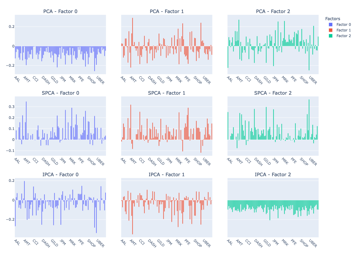
There are a few interesting things to note here, first PCA generates factors which are mostly expected. The first factor loads heavily on all assets (the market factor), and the others differentiate between assets. Furthermore, SPCA generates components which are fairly similar across the board, and there is no clear market factor. Finally, as for IPCA we can see the market factor in factor 3.

Factor Returns

Next, we look at the returns generated by our factors. In the first row we have the daily returns by the factors, and in the second the cumulative returns for each factor.

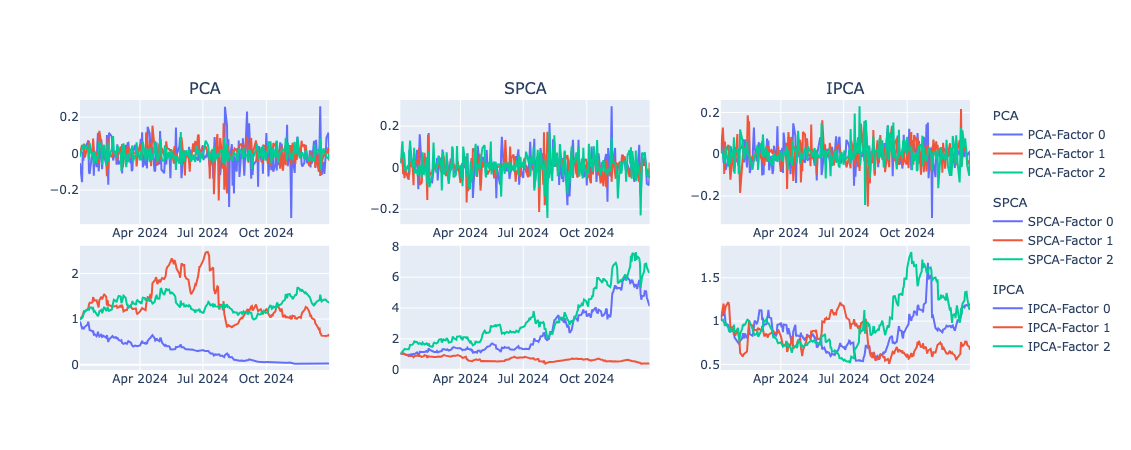
Again, we see similarites between PCA Factor 1 and IPCA Factor 3 in the cumulative return charts. Moreover, we can see that two of the SPCA factors perform very well over the period. This is reflective of the positive weights on these factors seen in the previous plot.

Idio Returns

Finally, we look at the idio returns by asset that are based on each of the statistical models.

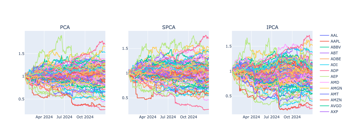
In contrast to the differences we saw within the previous two plots, the idio returns by asset appear fairly consistent across the factor discovery methods. This is perhaps more reflective of the fact that all of the factors represent the data well, but just in different ways.

Conclusion

To summarize, we first explored the formulation of the statistical factor models and then examined the use of different factor discovery methods. Finally, through empirical data we explored the differences in factor characterisitcs under each of these methods.

As always, you can find additional resources and code on my GitHub. Thanks for reading!

References

• (1) Paleologo, G. A. (2025). The Elements of Quantitative Investing. Hoboken, NJ: Wiley.